Lab 3: Wall Following on the Racecar

Check out our lab briefing here!

Purpose

Our team implemented a wall following algorithm for a racecar, as well as a safety controller to prevent any potential crashes if the algorithm fails.

Overview and Motivation

Our objective for this lab was to become comfortable writing programs for our racecar and to set the stage for more advanced tasks. The ability to follow a wall is an essential building block for navigation algorithms as it introduces basic path planning and motion control. For this reason, we programmed our racecar to follow a wall from a specified distance away. As our algorithms get more complicated, the environment becomes more hazardous, and our car starts moving faster, it is possible for our beloved - and expensive - racecar to crash. To avoid damage from bumping into obstacles, we have implemented a low-level safety controller that prevents the car from crashing. More specifically, it listens to the wall follower's commands and ensures that they are safe to execute.

Moving forward, the wall-following abilities of our racecar will allow us to optimize performance, particularly for speed and turning corners. Additionally, our safety controller will be essential in ensuring that we do not harm our racecar; not only is the it expensive, but damage to the physical components may hinder performance. By having a fail-safe that we can trust, we create more room for experimentation without worrying about crashing if we code something incorrectly. Through this lab, we have become comfortable with the ROS environment, implemented a wall-following algorithm, and programmed a safety controller to protect our racecar from damage.

Proposed Approach

Technical Approach - Wall Follower

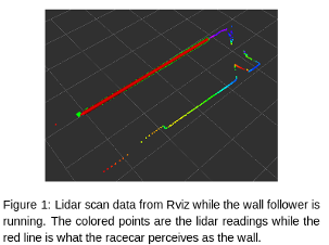
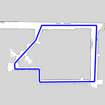
The foundation for our wall following algorithm is proportional and derivative control (PD). This feedback control responds to racecar's distance from the wall and the angle formed between the car and the wall. The wall is estimated using linear regression on points found in a subsection of the lidar scan data (Figure 1).

The distance from the wall and angle of the car with respect to the wall are calculated from this line, and the difference between these values and the desired values is the error that is fed into the control algorithm (Equation 1). The distance error is the proportional term (P) and the angle is the derivative term (D). The angle is considered a derivative because it dictates the rate of change in distance from the wall.

The PD controller uses the following formula to calculate the steering angle.

$Steering Angle = K_p \cdot (error \ distance) + K_d \cdot (error \ angle) \ \ \ \ \ [1]$

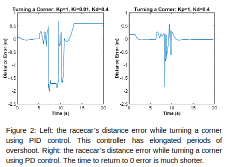
We decided to implement this PD controller instead of a proportional integral derivative controller (PID) because although adding integral control corrected for some imperfections in the steering angle, it also increased overshoot and added integral windup (Figure 2).

When we first moved from the race car simulation environment to the physical racecar, we ran into two main problems.

(1) The car followed lines that were not representative of the wall, causing wild oscillation.

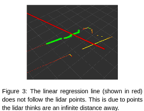
(2) When directly applying the simulation to real life, the regression lines were influenced by points outside the lidar's measurable range. This meant that the linear regression algorithm (from the scipy stats library) produced inaccurate lines (Figure 3).

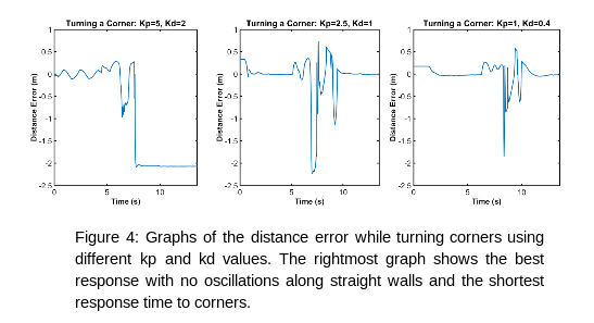
To correct this, we limited the points used for regression to those within 4.5 meters of the lidar. To minimize oscillations, we maintained the ratio of the proportional and derivative gains used in the simulation while experimentally testing smaller values until the oscillations minimized without compromising our ability to turn corners (Figure 4).

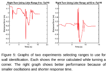
We also focused on deciding which portion of the LiDAR data was best for identifying the wall. While the range used in the simulation data, $\frac{pi}{30}$ to $\frac{pi}{16}$, worked well, we wanted to fine tune these values. After trying multiple ranges, we decided that $0$ to $\frac{pi}{16}$ provided the best performance. This range resulted in the race car turning tight corners the best (Figure 5).

Technical Approach - Safety Controller

If our wall follower algorithm fails, we need a safety controller to keep the racecar safe. Our safety controller operates by reading each high-level drive command, modifying it if the command is deemed unsafe, and publishing the modified command as a low-level drive command. Since our safety controller will be running for the rest of the labs, we want it to be robust to changes in speed, environment, and control systems. We also want to achieve a high standard of safety without limiting our car's abilities.

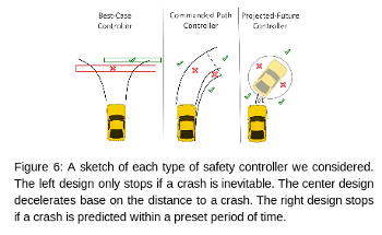
Our initial brainstorming sessions produced three potential algorithms for our safety controller: the Best-Case Controller, the Commanded-Path Controller, and the Projected-Future Controller (Figure 6). The Best-Case controller stops the racecar if and only if there is no possible path the racecar could follow to escape collision. The Commanded-Path Controller calculates the distance to the next potential crash and limits the velocity so that the racecar is able to decelerate before crashing. The Projected-Future Controller computes where the car will be at some time in the future given and if there is a collision at that time the car stops.

We selected the Commanded-Path Controller based on its robustness and conservativeness. We preferred the Commanded-Path over the Best-Case Controller because we felt the Best-Case Controller was too optimistic. The Best-Case controller assumes that the car will pick the best possible future path, while in reality we are concerned with scenarios where the path planner malfunctions. We also preferred the Commanded-Path Controller over the Projected-Future Controller. Although the Projected-Future Controller has an advantage when it comes to simplicity, it lacks robustness in that it does not adjust its behavior for different speeds or deceleration rates. The Commanded-Path controller is able to take these into account, allowing for more accurate collision prediction.

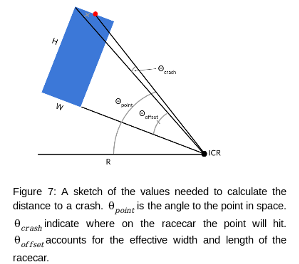
Here is an explanation for how the Commanded-Path Controller (Figure 7) computes the maximum safe speed for our racecar. First, we perform smoothing and filtering of the raw LIDAR data to minimize false positive detections. Then we compute the instantaneous center of rotation (ICR) from steering angle and chassis geometry. Finally, we trace out the path of both the front and the side of the racecar, recording the distance to the first collision with a lidar point. This distance is used to calculate the fastest possible speed that still allows the racecar to stop in time.

$Distance \ to \ Crash \ = \ R \cdot (\theta_p - \theta_c - \theta_o)$

$Max \ Safe \ Speed \ = \sqrt{2 \cdot deceleration \cdot distance \ to \ crash}$

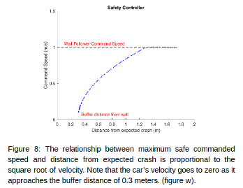
Our final safety controller algorithm includes two tunable parameters for flexibility. The first tunable parameter is the deceleration rate. This parameter can be adjusted when factors like the floor's coefficient of friction or the racecar's weight impact our ability to slow down. The second is a buffer distance which dictates how close the car can come to an obstacle before coming to a complete stop. In sum, our speed-limiting function computes the maximum speed our vehicle can drive at while still leaving enough room to decelerate to a complete stop before crashing.

ROS Implementation

All of our systems run on a ROS publisher/subscriber architecture via four main topics:

/scan This topic contains the output of the Hokuyo Lidar

/vesc/high_level/ackermann_cmd_mxu/output/navigation This topic is used by the wall follower to command the racecar to move.

/vesc/low_level/ackermann_cmd_mux/input/safety This topic is used by the safety controller to override the wall follower if necessary.

/vesc/low_level/ackermann_cmd_mux/input/teleop This topic is controlled by the remote control which can override all other commands.

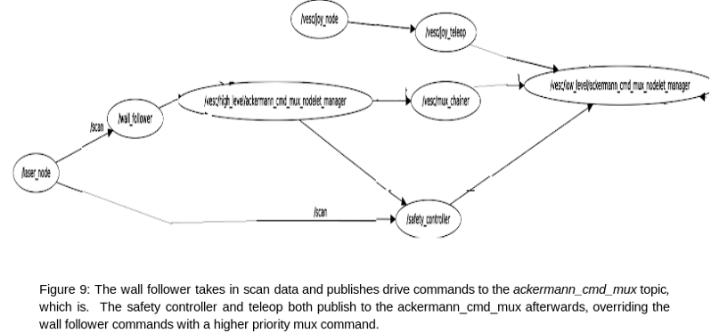
The mux architecture is a new idea introduced in this lab. At a basic level, mux is a built-in ROS node that can subscribe to a variety of topics and re-publish the topic of its choosing. In this case, the 6.141 TA's created a mux node that our controllers interface with, using the naming convention above. The purpose of the mux is to set priority levels for different control commands. For example, the wall follower and safety controller publish to a /vesc/high_level/ topic and a /vesc/low_level topic, respectively. The "low level" commands have a higher priority so that the safety_controller can override the "high level" commands sent by the wall follower. Similarly, the teleop topic has even higher priority so that we can always override the car's movement with manual control.

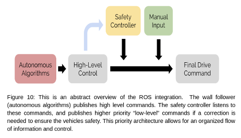
The control system is shown more abstractly in the figure below. The wall follower is the main code that moves the vehicle, making decisions based on the lidar data. The safety controller modifies the wall follower command if it deems the command unsafe. Manual input is used at the discretion of the drivers.

Experimental Evaluation

Testing Procedure

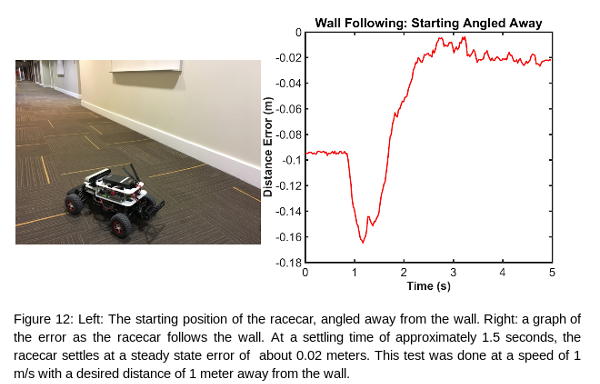
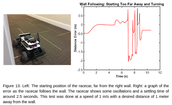
To test our wall following capabilities, we started the car parallel to the wall at the desired distance to see if it smoothly follows the wall. We noticed that we needed to tune the gains of our PD controller because the car wobbled about the desired path. After tuning the PD controller gains, we implemented more complex tests, starting the car at different distances and angles away from the wall, as well as testing its response at corners.

To test our safety controller, we tried to run the car into an obstacle at various speeds. We observed a jerky motion caused by the detection of obstacles that were not really there. This was due to the lidar detecting points on the racecar itself. To solve this problem, we limited the field of view of the safety controller.

Results

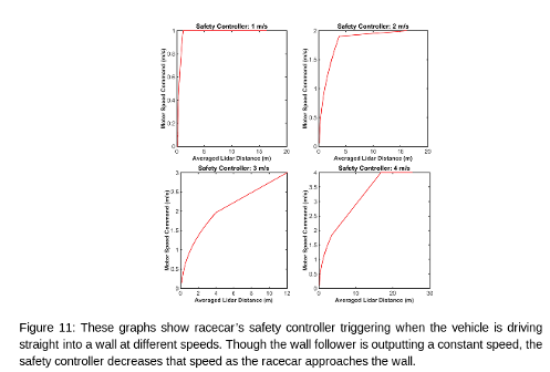
The safety controller gives the racecar ample time to decelerate and come to a stop at a threshold distance away from the obstacle ( 0.15 meters in this experiment). Once the racecar's distance from the wall decreases below this threshold, the safety controller reduces the speed to 0.

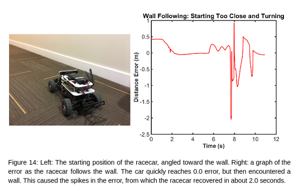
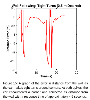
Overall, our racecar did well. It was able to follow all of the walls it was given, and was always able to recover from both wide and tight corners. For future improvements, we will aim to reduce the magnitude of the oscillations, as well as reducing the time it takes to reach a stable path.

Lessons Learned

As this was our first full team project, we learned a lot about the racecar platform, and how to approach a lot of different problems. Perhaps the most important technical skill we all learned was how to keep our code organized on Github so that everyone can stay up to date. We also learned about how the racecar responds to driving commands, such as steering angle and velocity, and how that differs from the simulation. These lessons allowed us to effectively parallelize our work and modify the existing codebase as needed.

Aside from the racecar itself, we learned a lot about our teamwork capabilities. Our strengths lie in our brainstorming sessions and using effective code structure. When brainstorming, we bring in a wide variety of ideas, and are open to discussing the advantages and flaws with each design openly. When coding, we have agreed upon an effective coding style that readily explains itself through docstrings and easy to follow variable names. However, there are certainly improvements to be made. We found ourselves diving into complex solutions, rather than starting simple and working our way up through iteration. Also, we were not perfect at communicating some technical details about how different parts of the code behave, such as what types of data to transfer and how the code will behave with different edge cases. These are things we are actively addressing now and look forward to improving in the future.

Future Work

In the future, we want to test our racecar's behavior under varying parameters, and document our experimental results for further improvements. Our wall follower and safety controller work well at slow speeds, but we have yet to test it at different velocities. In theory, our wall following algorithm should instruct the car to follow a wall at a high speed, and our safety controller should take over and prevent crashes no matter what speed we originally commanded. In addition, we will develop more qualitative results of our racecar's performance, such as recording the actual velocity versus the commanded velocity to find the actual acceleration of the racecar, as well as any delay times. This information will better predict the behavior of the vehicle and help analyze areas for improvement.

Lab 5: Localization

Check out our lab briefing here!

1 Overview and Motivation

Our team implemented a localization algorithm for an autonomous racecar, to enable robust state estimation using both sensor measurements and a known motion model.

When placed in a known environment, a robot still needs to figure out where it is in that environment. Localization is a method by which a robot can determine its orientation and position within a known environment. This capability is crucial for a robot when attempting to make decisions about future actions or paths to take. Localization is done by incorporating the information gathered from the sensors on the robot about the surrounding environment and its own motion in order to compute an accurate estimate of the location and orientation of the robot relative to the coordinate frame of the given map.

Computing the location and orientation of the robot within a map informs what drive commands are needed to reach a target. While previous labs have allowed the car to find certain attributes in an environment relative to itself, such as the wall and the cone, this will allow the car to find itself relative to the environment. When attempting to implement path planning algorithms, a robot will therefore be able to know its position relative to its final goal and devise an optimal path. With the racecar specifically, this will mean eventually being able to compute the optimal path ahead while racing in the basement of Stata.

2 Proposed Approach

The localization approach we used is divided up into two sections. Section 2.1 explains the algorithms we used for each part of the localization task. Then, section 2.2 gives an overview of the ROS implementation of these parts.

2.1 Technical Approach

Our approach to localizing the robot in its environment involves three main components: the motion model, the sensor model, and the particle filter. The motion model takes in odometry data, either from simulation or the actual robot, and outputs a cluster of particles that represent poses that the car could possibly occupy. Separately, the sensor model computes what the LIDAR scan data should look like for each pose in the cluster if the car was actually at that pose; it compares these model scans to actual LIDAR scan data and computes the probability of the car being in each position and orientation. Finally, the particle filter combines the results of the updated particles and computed probabilities to determine the most likely pose of the car. This pose estimation can be displayed on a map so we can estimate how accurate our implementation is on the robot. In simulation, we can calculate the error between where the car is and where it localizes to. The results of these tests will be discussed in the section 3 subsections. The rest of this section will detail each of the motion model, sensor model, and particle filter.

2.1.1 Motion Model

Often times we are not certain of the location of the racecar. The racecar may have been placed on the ground with a different orientation than expected, or may have drifted slightly while driving. One approach to this challenge is to consider many points where the racecar might be, and for each of these points, or particles, use exteroceptive sensors to determine the likelihood of it being the true position of the racecar. This models a distribution of where the racecar is likely to be, rather than assuming a single position with absolute certainty.

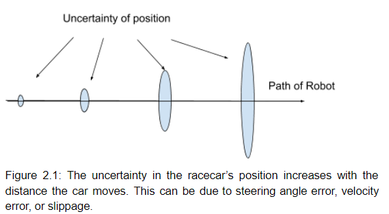
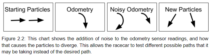
One advantage of this method is that it accounts for the sensor errors. For instance, when the racecar is commanded to drive at 1 m/s, it may actually be driving at a faster or slower speed. By adding random noise to the motion of the particles, we can have particles traveling faster than 1 m/s, and others slower. This ensures that at least some of the particles are likely to be traveling in the true direction of the car, so we have a much better chance of tracking its true position.

To implement this randomized motion, the racecar begins by creating hundreds of particles, each with an x-y coordinate and a direction. The points can all start at the same position if the starting position is known, or they may be spread out to cover a range of starting positions. The code then listens to the odometry data coming from the cars proprioceptive sensors, such as the encoders for the steering angle and the forward velocity. These values are assigned to the particles, each with a random amount of noise added. This noisy data is then transformed into displacement, causing the particles to each move in roughly the same direction while slowly spreading out, indicating the increasing uncertainty of the position of the racecar. The particles are then used in the sensor model for evaluation and pruning.

2.1.2 Sensor Model

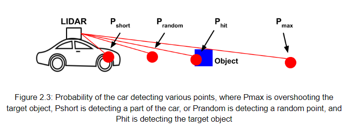
The sensor model is needed to accurately handle the inherent LIDAR noise and error, which can results in the LIDAR returning distances to “points” such as those shown in figure 2.3. Even though there is only one object, the LIDAR has a non-zero probability of returning other points such as overshoot the object, hitting a part of the car, or just another random point.

The sensor model was designed to handle fast and efficient computation of the probability that a given LIDAR value is accurate, given the previous position estimate and motion value of the car. Specifically, the model compares the LIDAR points observed by the car to the LIDAR points that should be observed if the car were at each of the particles in model.

Since each particle can have a large number of LIDAR values (~100 points) and there are sometimes hundreds of particles at a time, computing the probability of each lidar value every time requires significant time and computing power. With 200 particles and 100 LIDAR beams per particle, computing the probability of each value separately (in a for loop) takes about 0.30 seconds. Implementing the sensor model this way would limit the update rate of the sensor model to about 3 Hz if it were running on a laptop, which is too slow for real-time robotic control.

Thus, we decided on three key features to enable efficient sensor model computations:

• Precomputing the sensor model as a lookup table for a discrete range of possible LIDAR values.
• Downsample the laser scan such that fewer LIDAR points need to be compared on each pass.
• Implement all lookups using Numpy to ensure optimized computations.

Precomputing the model required discretizing a grid of possible ground truth values (zt*) and measured value pairs (zt) in the form (zt, zt*). For example, if the maximum expected LIDAR distance was 15 meters, we would create a matrix like the one in figure 2.4.

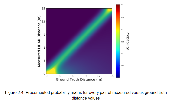
Determining the resolution of the table was a tradeoff between speed and accuracy. However, the LIDAR itself only has a accuracy of 6 cm, so we created a lookup table with 5 cm resolution which bounds the accuracy of our computations at the accuracy of the hardware. With a maximum range 75 meters, generating a table of probabilities from the (zt , zt*) pairs takes 0.65 seconds, but this only happens once when the car is turned on.

Additionally, each observed LIDAR point needs to be compared with a expected ground truth point. Thus, the number of beams per particle scales linearly with the number of LIDAR points that are used per calculation, which leads to a quadratic increase in the the size of the table. We downsample to 100 LIDAR points on each computation, which still provides enough comparison to get a good estimate of position.

<img src="/images/rss/lab5/table.png" alt=Table">

2.1.3 Particle Filter

The particle filter is structured to determine the most likely particle pose after utilizing the motion model and sensor model to generate particle positions and those particle positions respective probabilities. The particle positions and probabilities were fed into the numpy histogram built in to obtain weighted probability histograms. More specifically, three different weighted probability histograms for the x, y, and theta components of the particle poses were generated to determine the most likely particle pose. Once the three histograms were obtained, the peak bin for each histogram was taken as the most likely value range for that component of the particle pose; therefore, the peak bin boundaries were averaged to obtain a single value for the particular pose component. Below in figure 2.5 are examples of three histograms generated for the x, y, and theta components of the pose in the racecar simulation.

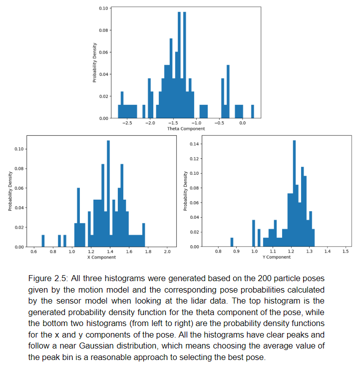
This histogram method was chosen as the best way to obtain a representative particle pose, because it is more robust than averaging since it disregards outliers that can heavily skew the data. This histogram method also eliminates the issue of attempting to find a weighted average of circular values for the theta component of the particle pose.

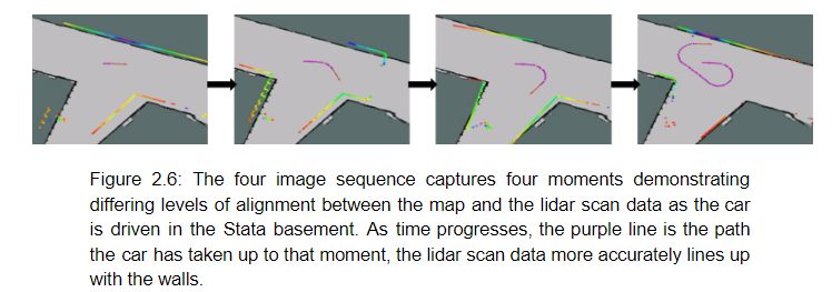
In order to initialize meaningful particles once the racecar is placed somewhere within the map scope, we generate a random spread of particles around a clicked point, which generates an initial pose, in rviz to set an initialize "guess" of the robot's position and orientation. Before the robot begins to move and while the robot is moving, the pose will update to better line up the lidar scan data based on the probabilities generated by the sensor model which correspond to the possible positions created by the motion model (figure 2.6).

The particle filter topic publishing rate is approximately 42 Hz when generating 200 particles with 100 LIDAR beams per particle. Therefore, the racecar pose is being published in real time (publishing rate of 20 Hz or faster). Having a publishing rate of 42 Hz means that if the car is traveling at 10 m/s, the estimated position will be around 25 cm behind the vehicle in the direction of travel, but this error can be minimized by inferring this lag based on current speed which causes pose estimates to be clustered in an area that closes this 25 cm gap.

2.2 ROS Implementation

The only rosnode implemented for this lab is the particle filter node, here named /particle_filter. Our particle filter node subscribes to the following topics, shown in figure 2.7: /scan, which provides the most current LIDAR sensor data /map, which provides a map of the domain /odom, which provides the most current vehicle odometry data /initialpose, which allows us to prescribe an initial pose using rviz

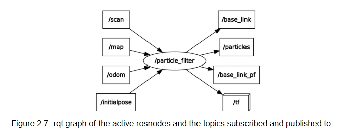
The particle filter processes this data with the help of the sensor model and motion model, which are implemented as python imports rather than separate rosnodes. Finally, the particle filter publishes to the following topics: /base_link, the most probable current pose /particles, an array of the particles generated by the filter at a given time /base_link_pf, the most probable current pose (published for plotting during simulation) /tf, which transforms between base_link and map frames according to the location of the car.

3 Experimental Evaluation

We tested our localization code in simulation and on the real racecar. Below, section 3.1 defines three scenarios we tested in simulation and the section provides numerical results and graphs for the error and convergence rates in each scenario. In simulation, we compared the estimated pose to the ground truth from the simulated odometry data.

The real racecar did not have a ground truth that we could compare our estimated pose to, so we relied on the rviz visualization of the inferred position in the known map. In section 3.2, we describe the scenarios that we tested and demonstrate the results of each.

3.1 Testing Procedure and Results: Simmulation

We gather empirical data on the performance of our localization algorithm in simulation, where we have access to the ground truth pose of the simulated car as well as pose estimate of our particle filter. We evaluate the performance of our localization algorithm in three different scenarios:

• Noise-free scenario: Evaluating localization in this setting allows us to verify the performance of the system in ideal conditions. We use the joystick to drive the car around the entire stata basement map in simulation, and plot the estimated x, y, and angle pose variables against the ground truth values in figure 3.1:

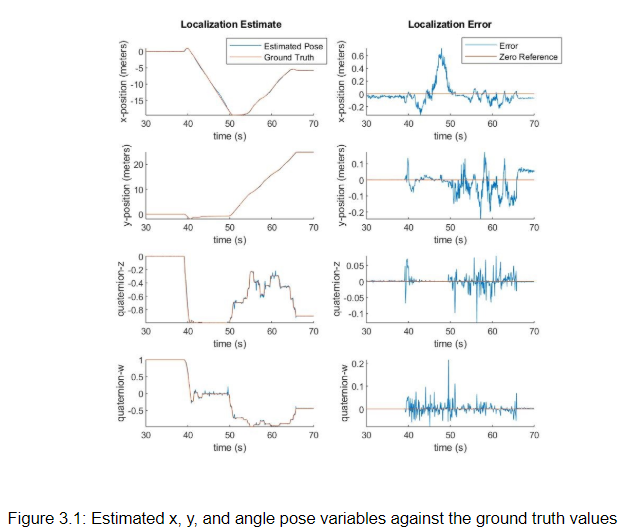
We observe that under the variety of conditions presented in the Stata basement map, our localization algorithm maintains a translational pose estimate within 0.1 meters of the ground truth and a quaternion rotational pose estimate within 0.1 of the ground truth. We believe these are adequate error margins for localization in a map of this scale.

The notable exception is when the x-position error of the car drifts to 0.6 meters between t = 45s and t = 50s. During this time the car is traveling down a long, featureless hallway along the x-axis. In such a hallway, the LIDAR scan would appear nearly identical at any x-position, so it makes sense that our particle filter would have trouble localizing precisely in this portion of the map. As soon as the car observes the end of the hallway around t = 48s, we can see from the data that the accuracy of the localization estimate is quickly recovered as the particles are re-weighted to match this observation.

• Noisy odometry scenario: We add random gaussian noise to the odometry reading from the car before it is passed to the motion model. Evaluating localization in this setting allows us to verify the ability of the sensor model to correct odometry error. To test, we drove the car straight in simulation. Each time a motion model update occurred, noise is drawn from a Gaussian distribution and added to all pose variables independently. The localization error and localization convergence for varying levels of noise input are depicted in figure 3.2.

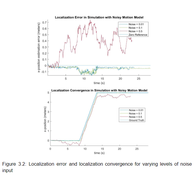
Our data illustrates that small and moderate odometry noise levels of 0.01 and 0.1 had negligible impact on localization accuracy. This demonstrates that for these noise levels, our particle filter is able to correctly identify particles close to the true pose of the car despite errors in the odometry signal. For a noise level of 0.5, very large random errors predictably caused particles to stop appearing near the true pose of the car, resulting in an inability to re-localize effectively using sensor data.

We could improve the ability of the particle filter to localize in the face of higher noise levels by increasing the density and dispersion of particle generation; however, this would come at a cost of increased demand for computation. Based on the performance of our particle filter on our real vehicle, our noise tolerance on the order of 0.1 in all variables is sufficient for our system in practice.

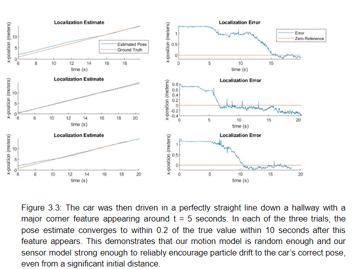
• Initialization error scenario: We provide the car with an incorrect initial pose estimate. This allows us to observe the convergence behavior of our particle filter. We initialized the pose estimate at some translational x-distance from its true position and observed how quickly the estimated pose converged to the true pose. In each of the three trials illustrated in figure 3.3, the initial pose estimate was set to 1 meter in the x-direction from the true starting position of the car.

3.2 Testing Procedure and Results: Real Racecar

To evaluate whether the car was localizing properly in the Stata Basement, we used rviz to visualize where the car was in four different scenarios. The first two scenarios were to test convergence when the car is moving or not moving. The last two scenarios were to test robustness to different speeds.

In order to test the convergence of the estimated location of the car, we set the car in an initial, incorrect pose and set the velocity to zero. We did this to test whether the sensor model would be able to update the particle positions and estimate a best pose without any significant change in odometry data. Next, we drove the robot to see if convergence would be faster or slower compared to the unmoving robot. We found that at standstill, the pose did start converging toward the actual position (we visually examined the robot and simulation environment to determine this), but driving the robot helped it to converge faster, as seen in figure 3.4. These results mean that having changing exteroceptive information and noise, and therefore better possible poses, leads to a faster convergence.

Figure 3.4: Initially the pose drifts to better line up the LIDAR data with the map walls without moving the racecar. Once the racecar is driven, the LIDAR data coverges to the map walls much quicker and more accurately.

We tested the scan data of the car at two different speeds: 1 meter per second (mps) and 2.5mps. At the higher speed, the scan data does not always correspond to what the estimated pose is; this is especially apparent during sharp changes in angle, like when turning. The videos of the car localizing at 1mps and 2.5mps are shown in figure 3.5. The lower performance at high speeds means that our car is unable to estimate reasonable possible poses in the motion model when the odometry data changes drastically in a short amount of time. We could try adding more noise to our motion model, or possibly make noise dependent on velocity.

Figure 3.5: The first two videos show the racecar and the corresponding rviz environment when driving the racecar in the Stata basement at 1 mps. The last two videos show the racecar and the corresponding rviz environment when driving the racecar in the Stata basement at 2.5 mps.

4 Lessons Learned

While implementing Localization algorithms on the racecar we made minor improvements to our coding style that have improved our time efficiency as a team. These improvements include making sure everyone is using the same indentation style and making sure to continue writing self-explanatory code via comprehensive variable naming and docstrings. This lead to our final code having little to no syntactic bugs that needed to be addressed.

Integration of the motion model and sensor model with the particle filter, however, set us back due to an error with certain file dependencies. This was a good reminder for us to make sure all of our files are compiled and up-to-date when attempting to run our code.

We also implemented a simple, straight forward solution initially before diving into more complex approaches. This has improved our time-management drastically as a team, and has allowed us to implement working versions of our code earlier on with minimal bugs, rather than spending most of our week debugging complex solutions.

5 Future Work

Our robot was able to localize itself within a known environment given the odometry data and LIDAR scan, but in the future, we would like to implement Google Cartographer on the racecar. This would enable real-time simultaneous localization and mapping (SLAM) on our robot so that we could localize in an unknown environment. Although we started working on configuring the Cartographer installation, we were unable to finish running and testing it by the deadline.

In addition to adding SLAM capabilities, we would like to test our localization algorithm at different velocities. At speeds higher than 2.5mps (the highest value we tested), its possible that the particle distribution would not spread out as much as necessary, and selecting the most accurate pose would be more difficult. We predict that at higher speeds, we will need to incorporate more noise. Furthermore, we plan to profile our code using a flame graph to understand and visualize where our code can be optimized. We were able to run our code at 40 Hz and did not find it necessary to optimize yet, but this tool will be useful in future labs.

Lab 6: Trajectory Planning Using A* and RRT*

Check out our lab briefing here!

1 Overview and Motivations

Across the six labs of Robotics: Science and Systems (RSS), we have gradually endowed our robot with abilities that have enabled it to operate more autonomously with each passing week. Our architecture has been true to the one introduced in the second lecture of RSS, visualized in Figure 1. In the first and second labs, we developed software for the low-level control and actuation of our robot. In the third lab, we developed low-level signal processing for our robot in support of our safety controller. As we advanced to the fourth and fifth labs, we moved up towards increasing levels of abstraction and autonomy in our robot's perception systems, implementing computer vision and localization capabilities. In this, the sixth lab, we make a similar step towards abstraction and autonomy, but this time in our robot's decision-making capabilities.

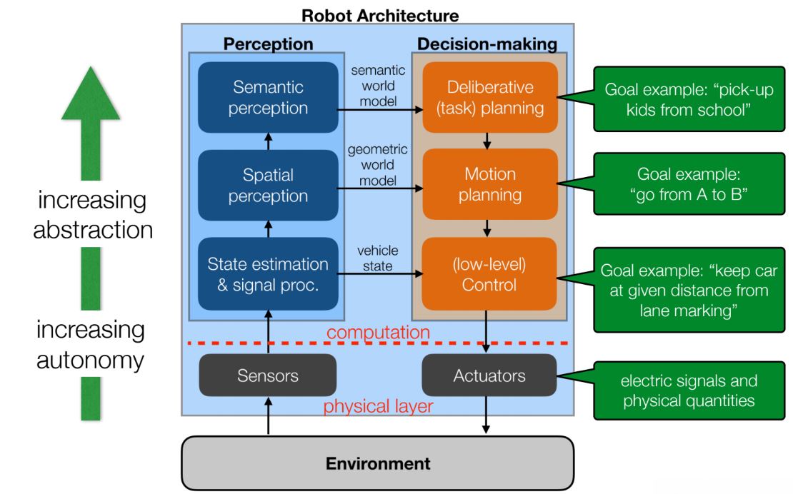Figure 1: The robot architecture introduced in Lecture 2 of RSS. The path planning system we implemented in lab 6 is a type of motion planning, a higher level of decision-making autonomy than we achieved in previous labs.

Motion planning is an essential ability for nearly any robot whose goal is to actuate change in its own state or the state of the world. Motion planning enables an autonomous agent that perceives its own state and is given some goal to string together a series of low-level actuation commands and arrive at that goal efficiently and safely. We use motion planning for our task of racing through the Stata basement, and enable our robot to generate a well-specified race plan given only its initial and goal states. Motion planning also finds application in the field of robotics more broadly. Particularly valuable is the application of robot motion planning to high-dimensional configuration spaces, as in the grasping movements of manipulator arms and the motion of other complex mechanisms with many degrees of freedom.

2 Proposed Approach

The challenge our team faced in this lab was to plan and execute a path between two randomly assigned locations. This path is judged by two metrics: the time it takes to generate the path and the time it takes to drive along the path. The sum of these two times was used to rate the quality of our path planning algorithms, with shorter times being better.

Rather than focus on just one type of path planner, our team researched and tested two distinct types of path-finding algorithms. This allowed us to compare the strengths and weaknesses of each, and to select the best one for final use on the robot. Our two approaches were a search-based algorithm, A*, and a sample-based algorithm, RRT*.

2.1 Technical Approach

One challenge of search algorithms is how to handle the physical constraints of the robot. For instance, a shortest-distance path will turn corners as tightly as possible. If the width of the robot is not accounted for, then the robot will clip the wall as it tries to turn. To account for this, we ran our path-planning algorithms on a dilated map. A dilated map expands walls and obstacles, limiting the search space to places where the robot can safely move without hitting obstacles.

Another challenge is developing a cost function, which is used to assign weights for moving from one position to another. Ideally, the cost function would model the search metric. For this lab, that would mean that the cost function is the time it takes to move between two points. Unfortunately, calculating this time is difficult because it is hard to know the exact speed the robot will be traveling, how much slip the wheels will have, how well the robot will follow the path, etc. For this reason, we chose to use distance between points as the cost function. While not ideal, this is a good approximation of the cost of moving from one location to another, especially if running the car at a constant velocity.

With a dilated map computed and a cost function defined, we implemented and tested two types of algorithms: search-based and sample-based. Search-based approaches discretize the map into finite locations and connect these locations in a graph. A search is then performed on the graph. Sample-based approaches instead randomly sample points on the map and build a tree that expands outward from the starting location until the desired end location is found. We tested both types of algorithms to compare both the speed of the search and the type of path that each produces. We then implemented a pure pursuit algorithm to compute steering angles in order to drive along our path. Sections 2.1.1 and 2.1.2 describe the algorithms and results of A* and RRT* respectively, while section 2.1.3 explains the pure pursuit method we used to follow our planned trajectories.

2.1.1 Search-based Planning

Search-based planning algorithms use graphical search methods in order to compute a trajectory between two locations. The input map for a search-based algorithm, therefore, must be a discretized grid representation of the map of the car's location. After considering the tradeoff between accuracy and computation time, we discretized the stata basement map with 20 pixel intervals. and every 20 pixels were defined as a point on the grid of pixels that the car was able to traverse to. Generally, the less pixels per discrete point that are assigned, the more precise the path can be; however, we determined that making the map more discretized than 20 pixel segments did not increase the efficiency of the planned path enough to outweigh the computational cost of running the algorithm with such a fine grid.

The search algorithm implemented on the race car is A*. Unlike other search-based algorithms, the defining feature of A* is that it optimizes the path it searches for based on a goal destination, only exploring possible paths that will lead closer to the goal, and leaving other areas of unexplored. The method by which A* does this is via a heuristic cost function dependent on the distance any single node is from the end node, in addition to a general cost function dependent on the distance it takes to get to the node from the start. The heuristic cost, or "Hcost", is defined as the euclidean distance between the node in question and the end node. The general cost, or "Gcost", is defined by the distance between the start node to the node in question. Figure 2 illustrates the logic of the A* algorithm implemented. The inputs into the algorithm are a start and end node, a grid map, and a discretization size for the grid map.

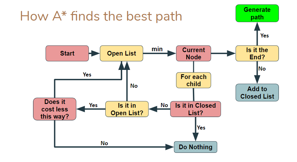Figure 2: Flow chart representation of the A* algorithm's logic. The algorithm begins by taking in a start node and feeding it into open list, which is a list of all of the nodes that we have seen/bordered, but not occupied. The node in this list with the minimum cost is then set as the current node, and for each child of that node, or the nodes that border that node, the algorithm goes through a series of steps to determine whether the child should be added to the open list. The algorithm terminates once the end path is reached and a path is generated.

After implementing A*, we also tried to optimize it for traversability and time, but it was too computational taxing. One method by which the A* algorithm implemented on the car could be improved is by modifying how the grid-based map input is discretized. Currently, the map is simply discretized into 2D x-y pixel locations. If the discretization had been expanded, however, into a 4D grid that also had the pose of the car and the velocity at any given location, only the children of each node that are physically possible to traverse would be considered; this would mean that the algorithm needs to traverse less of the map grid. Furthermore, the cost functions could then be calculated based on the time (rather than distance) it takes to get from the start node and to reach the end node. A time-based cost function would be much more ideal for this lab as the goal is to have the racecar traverse the Stata basement loop as quickly as possible, not in the shortest distance possible. While this 4D grid would be ideal, it was found to be too computationally demanding, and would not have provided enough of a significant improvement in the path generated by A*, at least for the application of looping through the Stata basement.

2.1.2 Sample-based Planning

In addition to A*, we planned trajectories with a sample based algorithm called RRT*, which is an extension to Rapidly-exploring Random Tree (RRT). First, we implemented RRT. To do this, we built a tree of paths rooted at our car's starting position. To add nodes to the tree, we sampled points from our environment and built branches in the direction of each point; we only added a branch if it was collision-free. Once a branch reached the destination region, we traced back up the parent nodes to construct the path. Figure 3 shows what our tree looked like after every 500 samples in simulation. The resulting path starts and ends as desired, but the path is jagged, hard-to-follow, and less than optimal. RRT by itself cannot find a more optimal path once a path is found, so we then implemented RRT*.

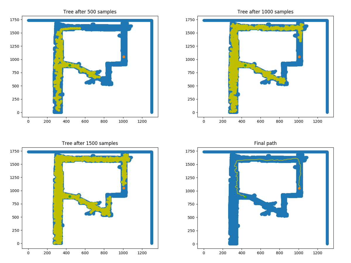Figure 3: RRT constructs a tree (yellow points, frames 1-3) through repeated sampling and expansion. Eventually, the tree grows into the goal region and a path is immediately returned (yellow line, frame 4). The final path contains evident jaggedness and is suboptimal.

For RRT*, we added a cost function based on distance to modify how branches were added to our tree. The reason we used distance as the cost function was because it would give us the best approximation for time, while being easily computable given our current graph; a longer path takes longer to follow, and we did not have to factor in states such as velocity to determine that. When a node was about to be connected, we checked nearby nodes within a "K" distance away to pick which one, if connected to, would result in the shortest path from the root to the new node. Then, all nodes in that range were re-checked and re-wired to shorten paths if a better possible path was found.

While writing both RRT and RRT*, we had to determine the best step-size, or length of each branch. If the step size was large, the algorithm found simple paths quickly, but was unable to find non-collision branches if the path was complicated. Smaller step-sizes were more reliable, but added to the computation time. We settled on a step-size of 20 pixels, or approximately 1 meter. Figure 4 illustrates the difference in path selected by RRT and RRT* respectively.

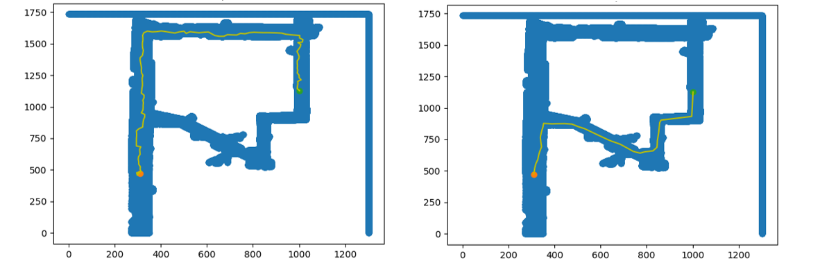Figure 4: The path generated by RRT is on the left, while the path generated by RRT* is on the right. RRT* plans a smoother and shorter path than RRT between the same start and goal points in the Stata basement.

2.1.3 Pure Pursuit Controller

Our sample-based and search-based planning algorithms each output a set of points defining a piecewise linear trajectory. We designed and implemented a Pure Pursuit controller to follow this type of trajectory. The Pure Pursuit controller identifies a point on the trajectory ahead of the car at some look-ahead distance, and steers the car along an arc that intersects that point (Figure 5).

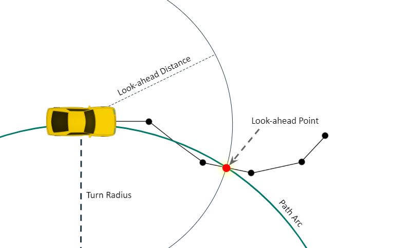Figure 5: Geometry of the Pure Pursuit controller. The controller computes a look-ahead path point at the prescribed distance and steers the car towards it.

The main design choice we made in our pure pursuit implementation was the selection of an appropriate look-ahead distance for our problem. In order to select an appropriate look-ahead distance, we evaluated the car’s cross-track error on a hand-drawn piecewise linear trajectory with several candidate look-ahead distance values. We found that for a look-ahead distance of 2.0 meters, the cross-track error was elevated, because the car did its steering based on a part of the path that was relatively distant from the car’s current location. For a look-ahead distance of 0.5 meters, we found that the racecar achieved low cross-track error but was susceptible to failure on tight corners because the controller would not begin to detect and follow the turn until it was too late to safely turn the corner. Figure 6 demonstrates the results of the described trials, and Video 1 visualizes our testing environment. We concluded that a look-ahead distance of 1.0 meter provided the best mix of low cross-track error and high robustness to corners in our simulated setting with a hand-drawn trajectory, and in section 3 we describe how we empirically validated that this look-ahead distance led to good performance in the real world.

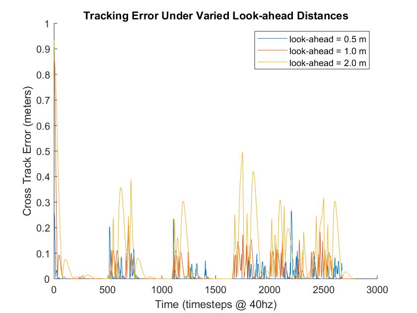Figure 6: We evaluated the effect of different look-ahead distances in the Pure Pursuit algorithm by tracking the Cross Track Error (XTE) to a planned path over the course of an entire simulated Stata basement loop. The longest look-ahead (2.0 m) resulted in higher XTE while the shortest look-ahead (0.5 m) lacked robustness around corners. A look-ahead of 1.0 m achieved both low error and robustness.

2.2 ROS Implementation

Our ROS implementation consists of five rosnodes: the Map Server, Safety Controller, Particle Filter, Trajectory Builder and Trajectory Follower, which interact with each other and the vehicle sensors and actuators through ROS.

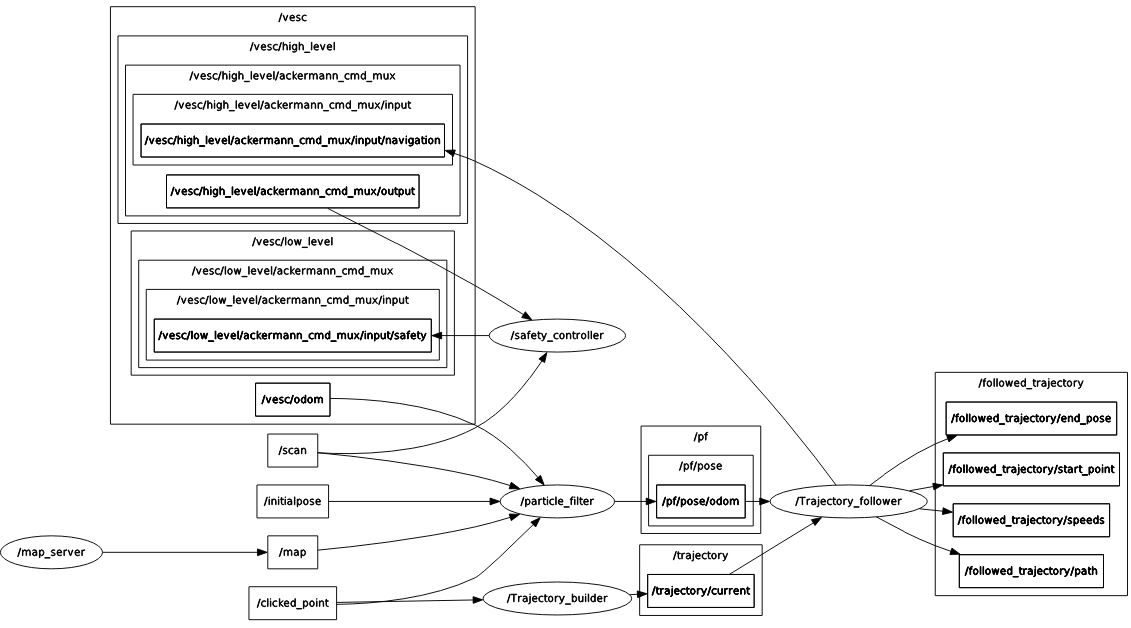Figure 7: The RQT graph of our complete path planning ROS implementation.

The flow of data in our ROS implementation is as follows: The Trajectory Builder subscribes to clicked points and publishes a trajectory between those clicked points built by either A* or RRT*. The Trajectory Follower subscribes to the path planned by the trajectory builder as well as the localization estimate of the Particle Filter (see Lab 5) and uses Pure Pursuit to compute and publish an appropriate steering angle and velocity to a high-level drive topic. The Safety Controller then evaluates the safety of this command based on the raw LIDAR sensor data before publishing it as a low-level drive command.

3 Experimental Evaluation

We tested both of our path planning algorithms, A* and RRT*, as well as pure pursuit in simulation; on the real racecar, we tested only A* and pure pursuit. Section 3.1 goes into depth on the test we performed in simulation to evaluate our sample-based and search-based path planning algorithms. The results of this test led us to decide to move forward with only our search-based algorithm, A*, on the real racecar.

In order to evaluate A*'s performance on the real racecar, we relied on the pure pursuit distance error: the distance between the car's localized position and the closest point on the generated path. Ultimately, this is not a ground truth comparison since this metric includes localization error, but it gave us a good estimate of how easy-to-follow our A* generated paths are in real life. Further evaluation was done by visually comparing the path the car followed in real life to the generated path visualized in RViz. In section 3.2, we go into depth on the real world test we performed and analyze a few videoes we took of the RViz and real racecar side by side.

Ultimately, the success metric of our racecar's performance is the ability to follow a path without crashing into obstacles, which our racecar is able to do at this point. However, after our real world quantitative evaluation, we concluded our racecar's path planning still needs future work to meet our desired performance for the full Stata basement loop.

3.1 Testing Procedure and Results: Simulation

In simulation we tested both algorithms using user-defined start and end point markers and evaluated the relative performance of the search-based and sample-based path planning algorithms using three different testing metrics: time needed to generate the path, path length, and pure pursuit error when following the path. The paths generated by the two algorithms can be seen in Videos 2 and 3.

In Videos 4 and 5, a demonstration of the simulated car following these paths using the pure pursuit algorithm can be seen.

As mentioned earlier, one of our test metrics is the pure pursuit error when simulating following the path. This error is defined as the distance (m) between the position of the simulated racecar and the closest point on the path. For the simulated tests shown in Videos 4 and 5, we plotted the corresponding pure pursuit path following error. The path following error for the same test with A* and RRT* is shown in Figure 8.

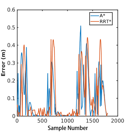Figure 8: The blue line shows the error for the A* algorithm, while the orange line shows the error for the RRT* algorithm. The peaks in error are where the simulated racecar is turning corners, which is where the racecar drifts away from the established path the most. For A* the average error while the path is being followed in simulation is 0.096 m. For RRT* this average error value is 0.103 m.

The main goal of this simulation test was to allow us to quantitatively decide which algorithm, A* or RRT*, we should use on the real racecar. This meant we wanted a path that was generated as quickly as possible with a reasonable path length that our pure pursuit algorithm would be able to follow with relatively low error.

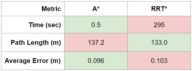
We decided a successful algorithm would generate a path of a reasonable length in ten seconds or less and that this path should be able to be followed with an average distance error of 0.3 meters or less. We decided to use ten seconds as the path generation metric because of the time limit of the checkoff of this lab. In this case, generating a path with reasonable length means a path that utilizes long straight lines when possible and does not backtrack or excessively zig-zag at any point in the path. Furthermore, we decided to use 0.3 meters as the cutoff for the average error because of the size of the buffer we used on the Stata basement map. Table 1 shows the results of the simulation test for both A* and RRT* in terms of the three testing metrics. Both algorithms were successful in terms of path length and average error, but RRT* was not successful in terms of the time it took to generate the path. This time could be brought down with further adjustment of the algorithm parameters, but we did not think this was necessary to pursue since A* was successful in all categories.

Table 1: The quantitative results of the simulation test in terms of our three defined testing metrics. Cells highlighted in green mean that algorithm performed better in that category, while red means the algorithm performed worse when compared to the other. It should be noted that the green and red highlighting do not represent the algorithm being successful based on our success measurements. A* was successful in all categories, while RRT* was not successful in the time category.

3.2 Testing Procedure and Results: Real Racecar

In evaluating A*'s performance on the real racecar, we focused on two main experimental metrics. The first was the pure pursuit distance error, the distance between the car's localized position and the closest point on the generated path. Secondly, we relied on visually comparing the path the car followed in real life to the path that was generated by A* in RViz. For example, we looked at how closely it cut corners in real life compared to the RViz path. It was necessary to make our own visual comparisons since the pure pursuit distance error is not a ground truth measure due to localization error. However, even though the pure pursuit distance error is not ground truth, it gave us a good estimate of how easy-to-follow our A* generated paths are in real life.

We tested using the pure pursuit error by following an A* generated path for the Stata basement loop, the same as for the final race. We ended up increasing the robot speed for this test in particular to ensure we could complete the loop in a reasonable time limit. Because our pure pursuit algorithm has not yet been modified to adjust properly for a differing racecar speed, our racecar excessively oscillated around the desired path. This oscillation can be seen in both the RViz visualization video and the actual racecar video in 6 and Video 7, respectively (both of these videos have been sped up to two times speed for viewing purposes).

Unfortunately, the RViz visualization froze at about halfway through the video in Video 6, so we cannot compare the RViz and the real world performance for the complete path. Despite these oscillations, the racecar was able to complete the full loop without any crashes, achieving our primary goal for path planning. We still need to modify our pure pursuit algorithm to eliminate oscillations even if the racecar speed is increased. This will allow us to complete the loop more quickly and effectively.

We gained insight into the car's performance and what needs to be improved from our visual comparison of the path and the racecar's movements. For a more quantitative metric to evaluate our car's performance, we collected the pure pursuit distance error based on the localization estimate of the racecar's position. This error is plotted in Figure 9. The average error for the loop was 0.87 meters, which is much larger than our desired criteria of success (0.3 meters or less). So while we were able to drive the path without any collisions, it is likely an inconsistent result that we cannot rely on due to high error. In order to have a successful real life performance for the entire loop, we need to modify our pure pursuit algorithm as mentioned earlier.

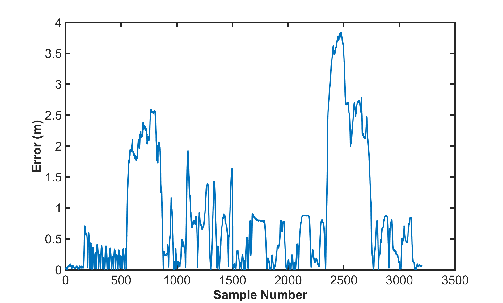Figure 9: The error for the whole duration of the Stata basement loop. There is a large amount of oscillation around the path, especially before 500 samples. The peaks in error are due to the racecar turning corners, which is where the racecar drifts the furthest away from the established path. While traversing the loop, the racecar's average error was 0.87 meters.

Since we used a faster speed then we had planned for our stata basement loop test, we used a slower, more reliable speed for testing only a portion of the Stata basement loop. For this shorter test, we did not collect the pure pursuit distance error data, but from visual examination, there were no significant oscillations. The RViz visualization in Video 8 shows that the racecar followed the path with very high precision, and there was little divergence from the path even when turning a corner. Comparing Videos 8 and 9 show us that there are no oscillations and the path is being followed as expected from the simulation.

As mentioned earlier, the overarching success metric of our racecar's performance is the ability to follow a path without crashing into obstacles. In both testing scenarios, we were able to do this, but we were not able to meet our pure pursuit distance error success metric when driving the full Stata basement loop. We will work on our pursuit algorithm so that it meets this metric for the final race.

4 Lessons Learned

The lessons learned from this lab extend well beyond search algorithms and ROS structures. As a team, we refined how we approached the lab, divided work, and integrated individual parts into a cohesive unit. One thing we specifically tried to emulate was our approach to lab 3, designing a safety controller. In that lab, we set aside time as a group to brainstorm ideas and approaches together before jumping into individual work. This structure kept everyone aware of the different parts of the project and allowed for more idea generation. This was useful in lab 6 when deciding between search algorithms and picking the cost function.

One new challenge we faced occured when migrating code from simulation to the racecar. In the past, this has been difficult but the one or two people assigned this task had always been able to make steady progress. In this lab, however, things worked out differently. We started with a mostly-working system with just one unknown bug. While debugging that problem, we regressed several times and eventually found ourselves unable to run any of the code on the racecar that had worked just hours before. To fix this in time for the final checkoff, we had to come together as a team, each trying different ways to fix the numerous problems. This led to a very tense, communication-intensive environment that we had not experienced yet. From this we learned how to approach the problem and work cooperatively on difficult bugs.

5 Future Work

Our work on the path planning lab enabled our car to navigate autonomously through the entire Stata basement after being given only a few waypoints. However, the class challenge is a test of time, meaning the robot's path planning, trajectory following, and localization have to be as efficient and optimal as possible. Moreover, our goal is to complete the course in record time.

The robot in its current state has inefficiencies in three criteria of path planning, trajectory following, and localization. Our initial ideas for optimizing path planning were based around a large graph representation for our search-based path planner - in fact too big for our computers to handle. Instead, incorporating orientation and velocity variables into our sample-based path planner will allow us to compute the most time-efficient path through the entire basement. Likewise, our pure-pursuit planner will be tweaked to find a better balance between error from the goal path and speed.

Lastly, the localization algorithms will be adjusted to better handle new objects in the hallways and higher vehicle speeds. A new map of the Stata basement may be constructed using Google Cartographer to provide the most up-to-date version of the environment to our vehicle. Additionally, the motion model and sensor model described in the Lab 5 report will be fine-tuned to propagate and select a high-quality position estimate. Overall, efficient and fast algorithms are what stand between our car right now, and the car that will win the class racecar challenge.

Final Challenge

Final Video

Final Video

Final Briefing

Final Challenge Briefing

Final Challenge: Navigating Using Deep Neural Nets: Gate Detection and Imitation Learning

1 Overview and Motivations

Each lab we have completed in Robotics: Science and Systems (RSS) has lifted our robot's autonomous capabilities up the ladder of abstraction: the safety controller dealt with low-level control and actuation, the parking controller lab worked with state estimation, and the localization and path planning labs involved spatial perception and motion planning.

Our final challenge consisted of two modules: Gate Localization and Imitation Learning. In the first module of our final challenge, we worked with the high-level perception capabilities of our robot, using machine learning to perform camera-based gate classification and masking. In the second module, we deployed an imitation learning system, PilotNet, which spanned low and high-level perception and control to drive a car around the entire Stata basement loop based solely on human-driven examples.

Deep learning for autonomous driving is a cutting-edge research field that many companies are investing in. Deep learning allows computers to learn from rich visual information about the environment in scenarios where explicitly model-based approaches are weak. Working on this final challenge gave us the opportunity to experiment with these novel approaches and understand how they work.

2 Proposed Approach

For each of the modules of our final challenge, we implemented a different machine learning approach appropriate for the task.

To perform gate detection, we needed to look at an image and determine if there was a gate, and if so, how to drive to it. This task is well suited for Convolutional Neural Networks (CNNs), which excel at object detection in images. A CNN works by performing a series of convolutions and pooling operations on an image to identify edges, shapes, and other features. By training a CNN on a labeled dataset (pictures labeled as having or not having a gate), we created a system which achieved multiple levels of abstract feature detection and identified the existence and location of a gate in a picture with high accuracy. From that information, we then calculated the necessary steering angle to drive through the gate.

For driving around the Stata basement, we used a different machine learning algorithm known as imitation learning. Imitation learning is a learn-by-watching strategy. One of the advantages of this approach is that it is simple to tailor a dataset to a specific application. The algorithm is given a dataset containing human responses to different situations. For instance, when given an image of a road curving to the right, a human will likely turn the steering wheel a certain amount clockwise. After training, the machine learning model will know to also turn to the right when given a similar image. To learn how to drive around the Stata basement autonomously, we first recorded several human attempts at navigating around the loop. Then, we used this data to train a model to respond in the same way.

2.1 Technical Approach

2.1.1 Gate Localization and Following

Image classification is a method that determines which of several classes an entire image frame is most likely depicting. Supervised learning with CNNs is an elegant and powerful method to produce accurate image classifiers in a variety of domains. In the supervised training of a classifier, training images are manually assigned one-hot labels indicating the class they belong to, and a CNN is trained to correctly predict the labeled class from all the pixels of an image.

Image segmentation, on the other hand, determines which pixels of an image belong to the same object as one another. Compared to classification, there is less consensus around the best technique to perform image segmentation. Fully supervised image segmentation using neural networks is a challenge, because labeling which pixels belong to an object in an image is a prohibitively time-consuming task for a human engineer to perform. Oquab et al. (2015) proposed a method for obtaining image segmentation ability ‘for free' from a well-trained CNN classifier, using a method known as weakly-supervised learning. Their insight was that the hidden layers of a CNN, which detect features in an image through convolutional and pooling operations, can function as an effective segmentation “heat map” in an image classifier, exhibiting high activation in the regions of the image where the object being classified is present.

We used a CNN-based perception module to localize gates using our racecar's cameras. First, we implemented a CNN image classifier to detect whether an image in our environment, the Stata basement, contained a gate or not. We trained our CNN using hand-labeled images taken by our racecar's camera in our test environment. Our “no-gate” data was generated by driving in the basement with no gate in sight, and our “gate” data was collected by driving with the gate visible to the car's camera. We collected 5500 “gate” photos for training and 530 for testing, and 5900 “no-gate” photos for training and 1200 for testing. Our CNN followed the LeNet-5 architecture (LeCun et al., 1998) with alternating layers of convolution and subsampling, as shown in Figure 1. We downscaled our images to a resolution of 240x320 pixels for input to our network. Our final network architecture (Figure 1) was as follows: Layer 1: Convolution, 7x7 kernel, 6 filters Layer 2: Avg-Pool, 5x5 kernel Layer 3: Convolution: 9x9 kernel, 16 filters Layer 4: Avg-Pool, 3x3 kernel, 16 filters Layer 5: Flatten to 1x3456 Layer 7: Fully connected 1x60 layer Layer 8: Fully connected 1x2 layer (output, steering angle and velocity)

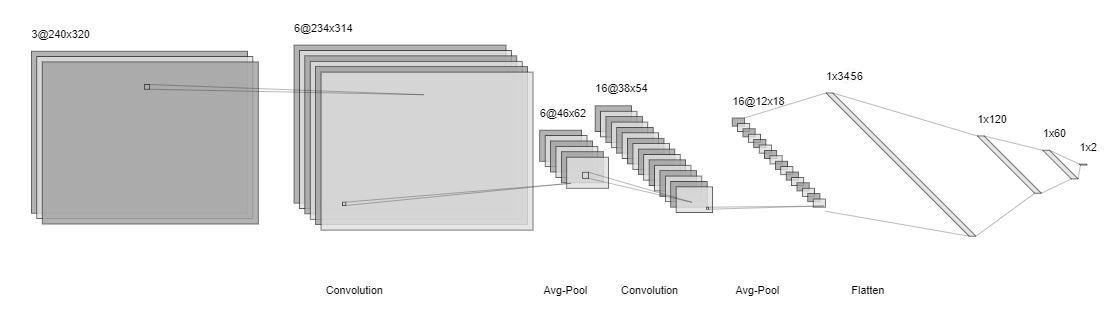Figure 1. Our CNN Architecture for Image Classification

Following the method of Oquab et al., we extracted a heat map from the final hidden layer of our architecture. Our network architecture was selected in part by tuning the parameters of our convolutional and pooling operations until the heat map we extracted was of appropriate resolution. The heat map generated from the architecture we selected was observed to align well with the true location of the gate (Figure 2).

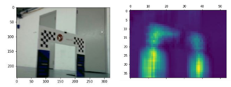Figure 2: Left: An image of a gate captured by our racecar's camera. Right: The heatmap generated by the activations of our CNN's final hidden layer. Activations are elevated (yellow regions) in the location of the gate.

2.1.2 Gate Navigation

With the heatmap generated by our CNN, our algorithm estimates the location of the gate relative to the racecar. We identified the point on the heatmap with the highest value and identified all points within a certain frame around the max point which achieved a value greater than 20% of the highest value. Also, we only look at pixels that are within 10% of the image height vertically from the y-position of max valued pixel. Essentially, we only analyze 20% of the image in order to reduce false positives - high heatmap values that correspond to non-gate features throughout the image. The pixel locations meeting both the 20% vertical zone requirement and the minimum 20% of the max value threshold were then used in a weighted average calculation to determine a “central” gate position the car should steer towards.

Our initial weighted average approach took three weighted averages: one for the left, center, and right image, assuming all three images were given a label of “gate”. These three weighted average locations were then averaged together to get a single pixel location. By performing three weighted averages followed by an unweighted average, we ended up with inaccurate central gate locations. The final location was both skewed by artifacts in the images that were not actually gates, but had high enough heatmap values to meet the 20% threshold, and by the fact that the cameras are mounted in an arc on the racecar. An example of this skewed data can be seen in Figure 4, which includes original and heatmap images.

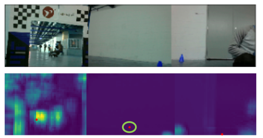Figure 3: (Top) Images from the left, center, and right cameras on the car. (Bottom) Corresponding heat map. The left image contains numerous false positives. The two non-circled red dots correspond to the center of the “gates” in the corresponding camera frames, even though there is no gate in the right image. The circled red dot in the middle is the average between the two red dots on the left and right, and it shows that the car will steer straight forward even though the gate is actually to the racecar's left.

After observing the lack of robustness in our approach, we decided on a new algorithm. We used the measured angles between the cameras, 45 degrees, along with the camera range, 60 degrees (Figure 4). We generated three angle ranges for the three different images to better understand the location of every pixel in the image. With respect to the car reference frame, the left camera covered 15 to 75 degrees, the center camera covered 30 to -30 degrees, and the right camera covered -15 to -75 degrees. We mapped the pixel in each image to a specific angle by dividing each individual angle range by the width of the image.

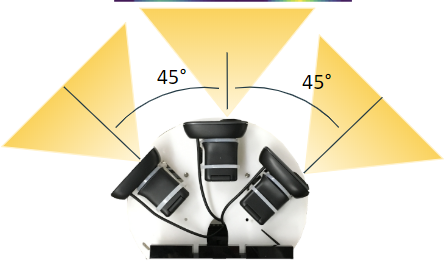Figure 4: The angle between each adjacent camera is 45 degrees when measured from the centers of the camera. The camera range for each camera is 60 degrees.

We then calculated the steering angle to be the single weighted average of angles, instead of pixel locations, using only the same pixels that met the 20% threshold and restricted vertical frame as described in section 2.1.2. The weights were defined as the exponential of the pixel's heatmap value, while the average over the corresponding angle values (in radians). We used an exponential function to intensify weight the high-pixel values of the heatmap. This generated steering angle was inputted as a steering command to allow the racecar to navigate through the gate. A successful gate navigation can be seen in Video 1.

Using deep learning for gate detection and navigation is a relatively novel approach, and we found it to have both strengths and weaknesses. Our CNN was accurate in determining whether or not there was a gate in the camera frame, which would have been much harder if we had used lidar scans to attempt to classify objects. On the other hand, it was difficult to generate a steering angle from the heatmaps that would work in multiple circumstances; we were not able to drive through more than one consecutive gate, and only certain starting positions enabled us to drive through the gate successfully.

2.1.3 Imitation Learning

Camera-based visual navigation is an appealing strategy for the control of autonomous vehicles. Cameras are currently less expensive than LIDAR sensors and can generally sense a more complete representation of the world. However, the control, localization, and mapping techniques we have implemented in past Robotics: Science and Systems labs for LIDAR-based navigation are not easily applied to camera-based navigation.

To address this, we turned to machine learning - specifically, we performed imitation learning with a CNN-based model called PilotNet. PilotNet learns from a dataset of images taken from example driving sessions. Each image is labeled with the steering command commanded by a human driver at the moment it was captured, and PilotNet learns to predict these labels in a generalized manner from camera images (Figure 5). We implemented PilotNet using the tensorflow machine learning library and applied it in two environments: the Udacity Self-Driving Car Simulator and the real-life Stata basement. After extensive data collection and tens of thousands of training iterations, we trained our implementation of PilotNet to map camera images to steering angles well enough to imitate human driving behavior, successfully navigating large segments of the Stata basement loop without human intervention.

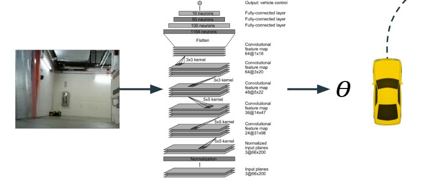Figure 5: CNN architecture for PilotNet model that we used for imitation learning.

2.1.3.1 Simulation Environment

To become familiar with how PilotNet reacts to changes in training data and other training parameters, we began our experiments in a simulated driving environment in the Udacity Self-Driving Car Simulator. We began by collecting four full laps of driving, during which the commanded steering angle is recorded along with left, right and center images from the perspective of the vehicle in the simulator. Video 2 illustrates the simulated vehicle being driven manually on the track.

Once data was collected, we began the training process. An important part of training is data augmentation. If a model were to be trained solely on the exact data we collected, the result would not be robust enough to small changes in conditions, such as the sun shining at a different angle or being on a different side of the track. Thus, we introduced randomly selected augmentations that essentially create formulated noise in the data. For the simulation data, this included increasing the brightness of the image, changing the gamma values, adding random shadows, and translating the image in various directions as seen in Figure 6. When our model subsequently encountered these conditions during deployment, it was better able to respond appropriately thanks to this augmentation.

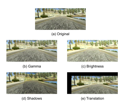Figure 6: Four different augmentations were applied to the training data to introduce noise. This improves the robustness to new data, as the model is presented with a larger variety of environments and training sequences.

The translation augmentation was an especially important transformation for this autonomous driving task because it enabled the model to learn what to do at a variety of locations on the track; the original data was taken from the car's location being close to the center the whole time, which is not always true during deployment. Our augmented dataset was used to train on the PilotNet model. We first tried training on 20 epochs of 300 images each, which led to a test accuracy of 78.7%. This model performed well on straightaways in the simulator, but failed on the first corner. After several iterations of data collection and training, the model eventually was able to complete half a lap as shown in Video 3.

2.1.3.2 Race Car: Table Path

Our next challenge following simulation was to train the car in real life. Before attempting to take on the basement loop, we traversed a simple path circling a table. This simple path was an appropriate stepping stone to the basement loop because it had an almost constant steering angle for the car to base its training on and no repeating features in different locations, allowing for a straightforward implementation of our trained model. Again, the training data we collected for our real-life driving tasks included the commanded steering angle of the racecar and the corresponding “long” image generated by the three cameras.

For the data to be useful to train a model for a moving vehicle, all of images in which the car was stationary (the speed was roughly 0 m/s) were removed from the training set. Following this filter, the images were randomly augmented to create a more robust training set for the model. The augmentations implemented in our model included random translations, horizontal flips, varying brightness, and changing the hue of the inputted images from the data set randomly similar to those in Figure 6 above.

After creating and training a model using the PilotNet architecture, running for 5 epochs at 800 steps per epoch, we validated the model on a test set and then implemented it on the on the table (Video 4).

2.1.3.3 Race Car: Stata Basement Loop

After a successful implementation of the model trained to circle a table, we began collecting data for the entire stata basement loop. Initially, our collected dataset was simply the result of three continuous laps manually driven around the loop. The training data and training methods for the loop was of the same format as described in section 2.1.3.2.

An apparent flaw in the trained model was that the model was able to follow straight paths in the long hallways very well, but failed to make even a single turn properly, as seen in Video 5. This was because our training data overwhelmingly consisted of examples in which the car drove straight, and our model was able to achieve low error without learning to take turns at all. To solve this issue, we collected more data for the turns and filtered out some of the straight path data to provide the car with a more uniform distribution of turning angles. This improved our models ability to make turns at all, but it was still unable to make the turns consistently.

In addition, we trained a model with just the data collected from the front camera to see if the steering angle offsets based on the relative angles of the side cameras to the center camera were the problem. Although doing so improved the model slightly, the improvement was not significant enough to be the root of our model's inability to make turns, so we returned to using all three cameras for training.

We finally achieved reliable turning behavior by implementing a variety of algorithmic improvements, like those shown in Figure 7. The first of these improvements was to shuffle the validation data, allowing the model to validate itself based on a random assortment of the training data, rather than simply the last batch of data collected, allowing for a better distribution of validation steering angles and resulting in better quantification of our training progress. Furthermore, we switched to a Mean Absolute Error rather than a Mean Squared Error as as our loss function which made out model more robust to outliers in our data. We also collected a larger quantity of data, including a lot more turn data, and supplemented it to our previously collected data set to increase the set of data to train the model on.

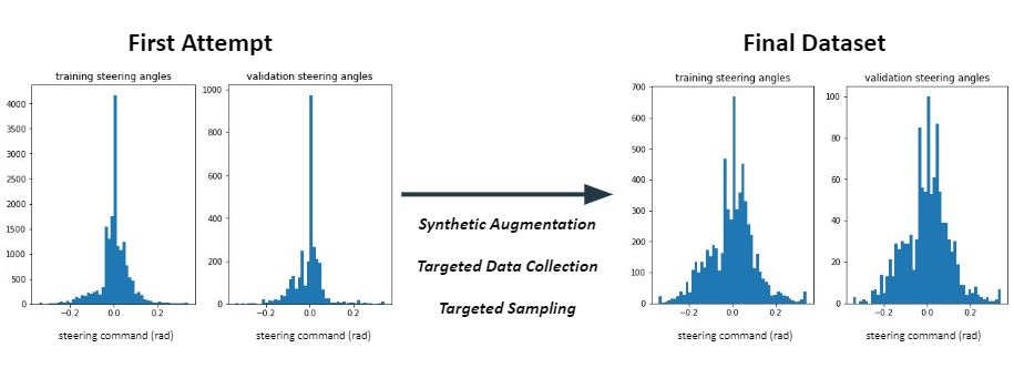Figure 7: Through a variety of solutions, including image augmentation, targeted data collection, and targeted data sampling, our training model was provided with a more uniformly distributed set of steering angles, enabling it to learn diverse turning behaviors.

Lastly, to reduce the test loss and training loss of our model, we trained for more iterations than we had previously attempted. This was to provide the model with ample ability to converge to a global minimum for its loss.

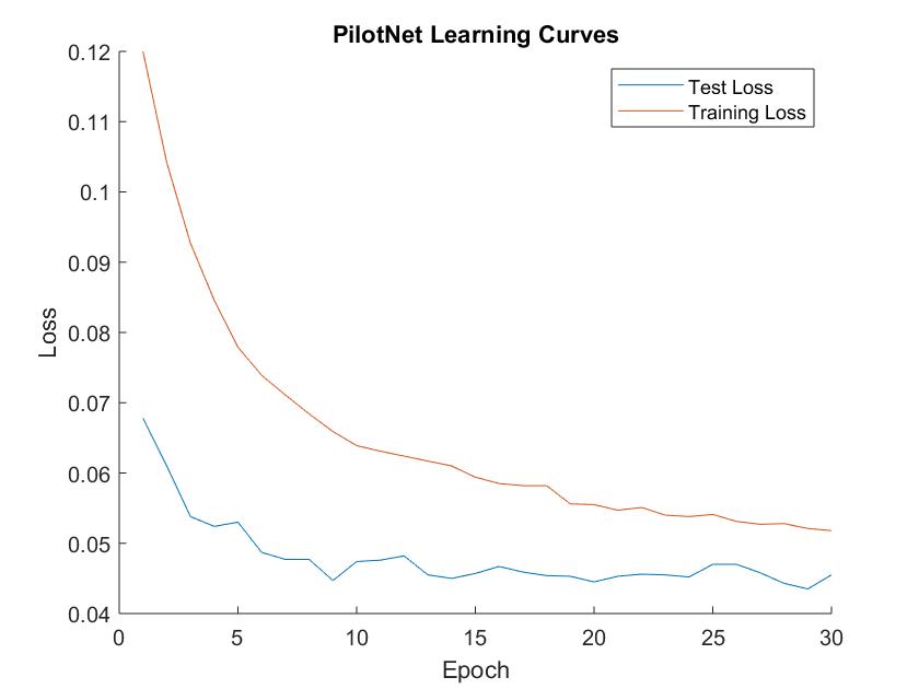Figure 8: Loss when training for 30 epochs at 2000 steps per epoch; stability is nearly reached at 20 epochs.

After training the model for more than 30 epochs at 2000 steps per epoch, as seen in Figure 8, we found that the model's validation loss began to level out at approximately 20 epochs, and so we deployed the model obtained with 20 epochs of training.

2.2 ROS implementation

The majority of the work for the final challenge was done in Tensorflow, but interaction with the low-level control software of the racecar was also necessary to actuate the neural network's commands. Tensorflow and the rest of the image processing stack ran in Python 3, while ROS runs in Python 2, so a workaround to communicate between the two languages was required.

The ZMQ library is a Python 2 and 3 library that allows for simple networking. Essentially, a local Python 3 server was created to capture image data and infer the correct steering angle from the model. A Python 2 client would listen to this server and frequently request the steering angle. In this manner, a ROS Node was able to command a steering angle and drive speed while the neural network was working in parallel, which is noted in Figure 9.

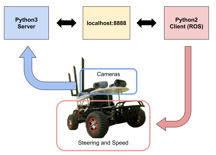Figure 9: The Python 3 server runs the neural network inference model and sends the required steering angle to the ROS nodes via a local network. ROS controls the steering and speed, which in turn updates the location and camera feed of the car, and the cycle continues.

Although the Python 3 server was chosen to capture image data from the cameras, ROS could have also been used to capture image data into ROS topics and transport it between various nodes. However, since no other nodes required the image data, it made the most sense to have the Python 3 server handle all the image capture itself.

3 Experimental Evaluation

Due to the nature of machine learning, it is difficult to quantitatively evaluate our performance when testing our generated models. Unlike path following with LIDAR-based localization, there is no ground truth value to compare an action to. Instead we have to rely on an understanding of what actions seem justifiable and make situational sense based on the given application. With this in mind, we evaluated our models' respective performances in three ways.

First, we evaluated our model performance based on the model's accuracy on the data training set. A model's training set performance was deemed adequate when the accuracy was within 90% to 95%. Although training accuracy is not always a great indicator of real-world performance, an accuracy above 95% for the models we used generally would have indicated overfitting, so we didn't want to surpass that.

Secondly, after performing well on the training set, we evaluated our model on a test set. A model was expected to achieve an accuracy between 75% and 85% on a validation set in order to be considered a successful model that could be applied to the desired environment.

The third and final method of evaluation occurred when testing the model in the proper environment: the environment being either simulation or the real world based on the desired model application. The evaluation method used is essentially based on the model's ability to complete the task at hand: navigation through gates and traversing an imitated path without crashing or going off course. While this evaluation is not numerically supported, it is the most important form of evaluation since the end goal is to successfully complete the desired task. This evaluation method often differed from the expected results based on test accuracy, showing that there was still a lot to be understood about how the model learns features.

3.1 Gate Detection Navigation

Our best performing gate detection model has a training accuracy of 93%, which is within the successful range of 90% to 95%. Unlike some of our other models that overfit the training data and performed poorly on the test set and in real life, this model had a reasonable accuracy on the test set as well. The model test set accuracy was 81%, which is within our desired range of 75% to 85%. Since our model met our first two success requirements, we moved onto the real world implementation.

We achieved varying results when evaluating the real world application of gate detection/navigation on the racecar. The racecar was usually able to find its way towards the gate, but often crashed into the leg of the gate instead of navigating through it: both scenarios are seen in Videos 6 and 7.

Less than half the time, the racecar was not able to navigate towards the gate at all. This occured when our heatmap picked up on parts of the environment that were not the gate. Ultimately, our model relies on deciding if the image has a gate in it by detecting the columns of the gate (Figure 10). As soon as a person or other column-like object was detected in the camera view, the model (often incorrectly) indicated that the column object was a gate. This improper identification resulted in an inaccurate steering angle away from the actual gate.

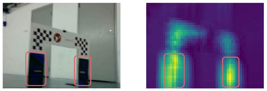Figure 10: The model identifies columns as gate features, even if the columns are not actually part of the gate. Here, the model correctly detects the gate supports as the gate itself, but other columns or people in the hallway often confused the model.

Despite the pitfalls of the model and its sporadic ability to navigate through gates, the model performed as expected and can be deemed a success. Since we are using weakly-supervised learning with a binary classifier, we cannot expect 100% accurate navigation; we can expect the model to do a good job at classifying an image as having a gate or not having a gate, but we cannot expect the model to fully understand all the features that make up a gate. We are using an early and outdated machine learning approach, so we did not expect as high level performance as can be achieved by some newer deep learning models. Additionally, our model is only using two convolutional layers, which limits our performance. The fact that our model had high accuracy in classifying the existence of gates and was able to allow us to navigate through gates a portion of the time is a great success considering the limitations of the model implementation.

3.2 Imitation Learning: Simulation

The performance of the simulation was evaluated based on the ability to stay on the simulation track and complete a lap. Although the car never completed a full lap, the performance improved as we iterated on the training parameters. Surprisingly, the simulations models all stayed around 80% test accuracy, even though the autonomous simulation results improved qualitatively (the car travelled farther). This could be the result of a variety of factors, but primarily the model may not have learned the correct features each time, such that it coincidentally was doing the right thing until it failed.

When we began increasing the number of images in an epoch from 300 to 1000, we saw drastic improvements in the simulation results even though the test accuracy was still at 78.6% in our most successful model (compared to 78.7% for our first model). At the same time, we were also including more corners in our data so that the ratio of corners to straightaways would be higher. Although the test accuracy did not improve dramatically, the performance of the model in simulation suggest these changes produced a better training environment such that model learned features that more directly correlated to simulation track performance. Further improvements could be made by quantitatively analyzing the distribution of data and steering angle in comparison with simulation results, such at the analysis done in Section 2.1.3.3 for the full basement loop.

3.3 Imitation Learning: Real World

The initial model performance was evaluated based on both the comparison between the validation set steering angles and the training model steering angles. This, however, was not the final method of evaluation, as the true test of the model's performance is its ability to traverse the path it is trained to in real life.

In the first simplified training environment, which involved circling a single table, our model was able to successfully traverse the circular path because of its simplicity, but more refinement to our training algorithm was needed in order to train a model on the stata basement loop.

For the second model, which navigated the entire stata basement loop, the improvements to the training algorithm mentioned in Section 2.1.3.3 resulted in a very robust training model that was able to adequately traverse the Stata basement loop.

4 Learned

The final challenge taught us many important lessons that we are sure to use in our future work in robotics. Because this challenge was so dissimilar to past labs (because it focused on machine learning), the learning curve was steep and it took us some time to get situated with the implementation and testing environments.

First of all, machine learning, especially with pre-made NN architectures, can often be blackbox that is hard to debug. The exact mechanisms for learning features and actions are not entirely understood. There were times that we got stuck and had to turn to each other to brainstorm solutions to fix the issue. Additionally, collecting training data often takes time, and this process has to be repeated as we learned more about what type of data the model needs. This is especially true for the PilotNet model, because imitation learning is only as good as the data collected, so having a method of collecting consistent and useful data was critical in achieving success.

Furthermore, we began to understand the limitations of hardware when we tried training on computers without GPUs; it's important to consider the operating machine when implementing algorithms that involve a lot of data processing. Finally, we learned better time-management techniques when it came to splitting up work, because we had three separate, time-consuming tasks (gate detection, imitation learning, and final race). At first we have everyone try to work on the challenges, but eventually moved two people to work fully on the race.

5 Future Work

Looking forward, we would like to delve into reinforcement learning which is a trendy topic in autonomous robotics right now. Throughout the final challenge, we were implementing supervised learning, that is, learning based on the guidance of the inputs, which have been labeled to serve as “ground truth” of what is correct. For small datasets, this generally works well, but as models get more complex and more data is needed, gathering and labeling large sets of data efficiently and accurately is a logistical challenge. Instead, reinforcement learning can be used to learn faster and more accurately.

For the scope of this class, we attempted to train the car to drive around the loop simulator similar to what we did with the imitation learning. However, instead of training on our own laps, we would start the car with no prior information, and give it a “reward” for staying in the middle of the track. If it ever leaves the track, we would restart the training, while keeping the information the car had already learned. Thus, over time it would learn that the best possible “reward” could be achieved by steering to the middle of the track from the entire loop. One of the biggest benefits of this approach is that it can be done quickly, as driving can be done at an accelerated speed, rather than making a human drive around the track each time more data is needed.

Although an area of active research, we could further this work by attempting to transfer the reinforcement learned model from the simulator to the vehicle. However, a much more accurate simulator for vehicle dimensions and environment would have to be used, and many refinements would have to be made to the model once it was on the vehicle.